Differential Equations

In single maths, first-order differential equations are the only ones looked at, and are solved by separating the variables:

When dy/dx = f(x) g(y), you can say ∫ 1/g(y) dy = ∫ f(x) dx

• Move all the y terms to the left where the dy is

• Move all the x terms to the right, including the dx

This allows you to integrate each side with respect to the variable on that side to solve the equation.

• You only need to add the ' +c ' to one side.

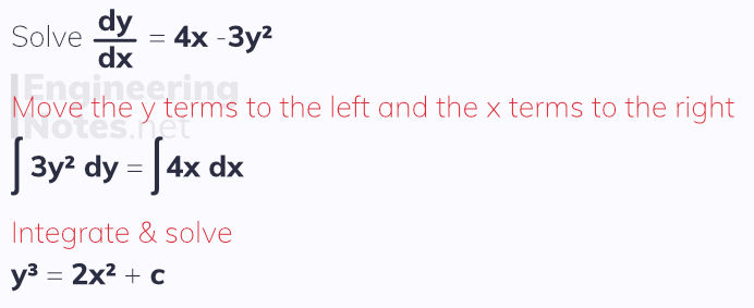
Just like when integrating an indefinite function, the initial result is a general solution and could be anywhere along the y-axis (see section on indefinite integral functions above). To fond the particular solution, you need to know a coordinate point on the curve - sometimes this is called a boundary condition.

Integrating Factor

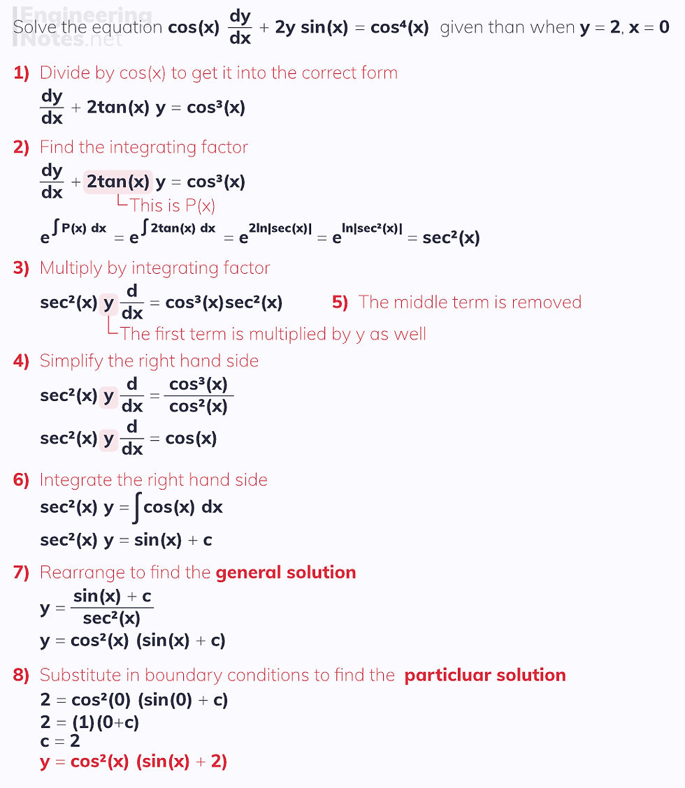
This is not covered in single maths, but is an important method of solving first-order differential equations where x and terms are multiplied by one another in one of the terms:

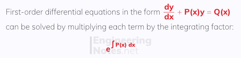
1. Rearrange to be in the form dy/dx + P(x)y = Q(x)

2. Find the integrating factor using the formula above

3. Multiply the dy/dx by the integrating factor and by y

4. Multiply the right hand side by the integrating factor & simplify (if you can)

5. The middle term, P(x)y disappears

6. Move the dx to the right hand side and integrate this side

7. Rearrange to make y the subject - this is the general solution

8. Find the particular solution by substituting in boundary conditions (if there are any)

At further stage, we also look at second-order differential equations - these come in two types: homogenous and non-homogenous.

Second-Order Homogeneous Differential Equations

Second-order homogeneous differential equations can be solved when in the form:

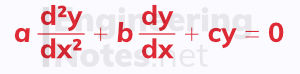
Homogeneous means it equals zero

The solution in terms of y will have four constants that need to be found:

• λ and μ, which are found by solving the auxiliary equation

• A and B, which can only be found if you have boundary conditions

The auxiliary equation is am² + bm + c = 0, and its solutions are λ and μ

• a, b, and c are the coefficients in the second-order homogenous differential equation above.

The format of the solution in terms of y depends on the auxiliary equation:

Second-Order Non-Homogeneous Differential Equations

Second-order homogeneous differential equations can be solved when in the form:

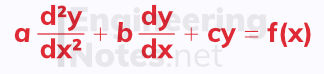
• The left hand side of this equation is known as the corresponding homogeneous equation and its solution is called the complementary function.

• The right hand side of this equation is a function of x and its solution is called the particular integral.

Non-homogeneous means the corresponding homogeneous equation equals a function of x

To solve a second-order non-homogeneous differential equation, first solve the corresponding homogeneous equation as normal (see above), and then find the particular integral:

1. Take the correct standard function

2. Find dy/dx and d²y/dx²

3. Substitute these into the initial equation

4. Solve to find the constants in the standard function

The form of the standard function depends on the form of f(x):

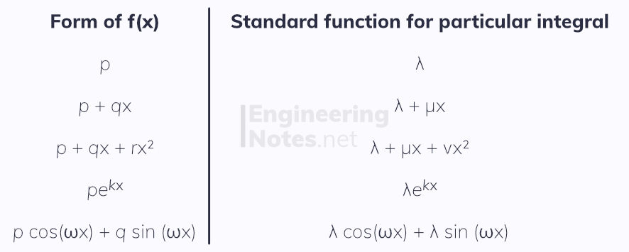
When the particular integral is already in the complementary function, you need to multiply the particular integral by x

For example, if f(x) is in the exponential form where k is the same as one of the roots in the auxiliary equation, multiply the particular integral by x.

The complete solution to the non-homogenous second-order differential equation is given as the sum of the complementary function and the particular integral:

Solution = complementary function + particular integral

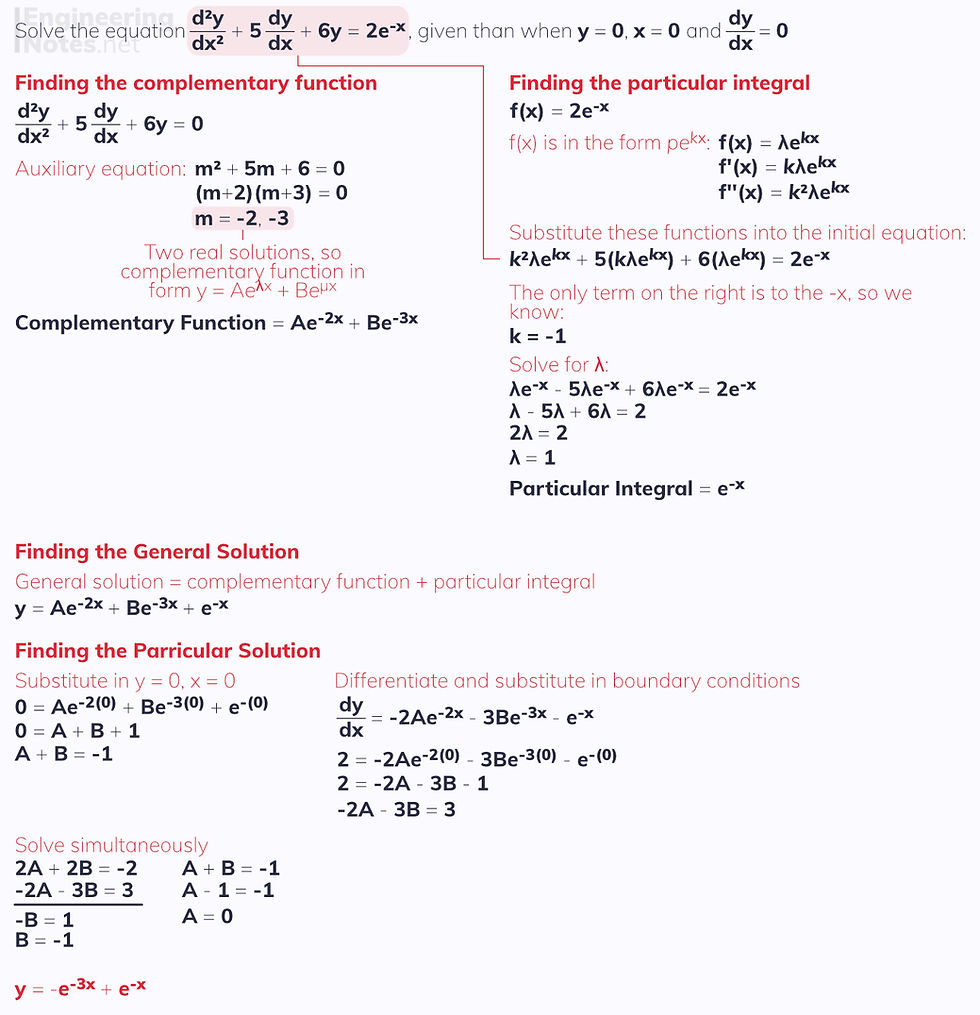
• Note that in this example, the exponent in the particular integral is -x. If it were -2x or -3x, it would be the same as the solutions to the auxiliary equations, so we would have to multiply the particular integral by x.

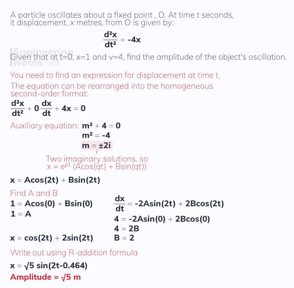
Simple Harmonic Motion

Simple harmonic motion (SHM) is when a particle always accelerates to a fixed central point (or origin) on its line of motion. The acceleration is proportional to the displacement of the particle from the origin.

It may be useful to check out the notes sheet on SHM from A-Level Physics before reading on.

SHM can be modelled with second order differential equations, because:

• x is displacement

• v is velocity, displacement with respect to time

• a is acceleration, velocity with respect to time

Therefore:

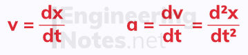
Often, we represent this with dot notation, where the dot above a variable means that that variable is differentiated with respect to time.

Since the acceleration is always proportional to displacement, and always directed to the origin, O, there must be a negative constant of proportionality. This is called the angular velocity, and is represented by ω².

Terminology

• Amplitude is the maximum displacement of the particle from the origin

• Period is the time taken to make one complete oscillation: this is from the origin out once, through it again to the other side, and then back to the origin.

• If an object is oscillating, this generally means it is moving with SHM

R-Addition Formula

When x is given in the form A cos(ωt) + B sin(ωt), it can be written as r sin(ωt - α). Here, r is the amplitude of the SHM, and is found as:

• r² = a² + b²

• tan(α) = A/B

Damped and Forced Harmonic Motion

Harmonic motion is only simple if there are no external forces slowing it down or speeding it up.

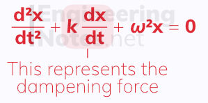
Damping

If there is an external force slowing down the motion of the particle, it is known as a dampening force. This is modelled by second-order homogeneous differential equations with a dx/dt term in the middle:

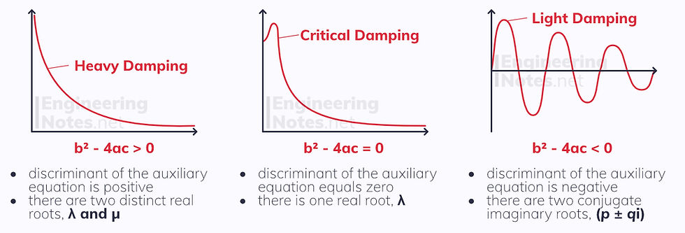
There are three separate cases, depending on the discriminant of the auxiliary equation:

Forced Motion

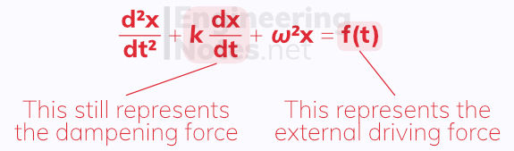
If energy is being put into the system, and the oscillating object is driven by an external force, it can be modelled with second-order non-homogeneous differential equations:

Questions relating to these contexts are solved exactly as any second-order differential equations should be solved.

Coupled First-Order Simultaneous Differential Equations

Often in nature, the rate of change of one thing is dependent on the rate of change of another thing. A common example is how the population size of predator affects that of the prey, and vice versa:

• If the population of rabbit is large, the population of foxes increases

• If the population of foxes is large, the population of rabbits decreases

In such an example, there are two variables (one for the size of each population), and so there are two differential equations to represent how each changes with respect to time. Naturally, these can be solved simultaneously.

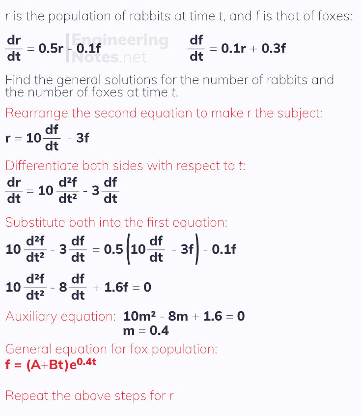
If r is the number of rabbits at time t, and f is the number of foxes at time t, we can write:

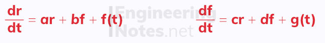
If both f(t) and g(t) equal zero, the system is homogeneous.

To solve coupled first-order differential equations, you need to eliminate one of the variables.