Control Volume Analysis
- Engineering

- Dec 1, 2020
- 4 min read
Updated: May 19, 2021
In this notes sheet...
As seen in thermodynamics, there is a difference between systems and control volumes. The former are used for a fixed mass of fluid, constantly moving, the latter are used for fluid flow through a defined boundary.
We hardly ever model a fixed mass of fluid, and as such we always use control volume analysis in fluid dynamics.
Mass Flow Rate
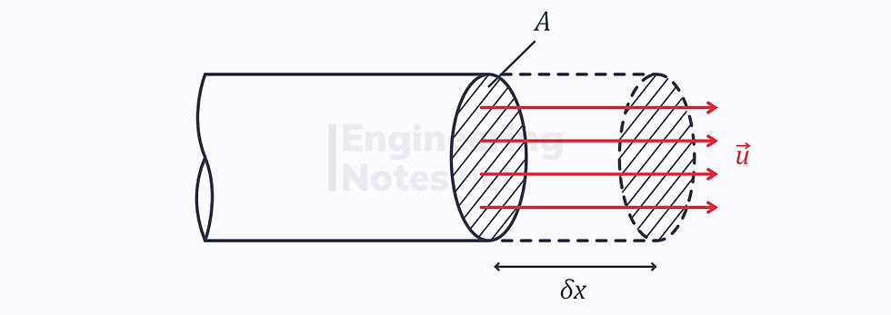
Over a set time δt, a distance δx is travelled by any given fluid particles. Therefore, the swept volume over time δt is Aδx. This volume has a mass, ρAδx.
The mass flow rate is the derivative of this with respect to time:

This can be re-written in terms of normal velocity, u:

Mass flux is another description of flow, given as the mass flow rate per unit area:

The velocity must be normal to the area.

If the velocity is not normal to the area, δA, we need to find the normal component as the scalar product of the velocity and normal vectors:

Writing δA as a vector:


This is the most important equation for mass flow rate. It will crop up in the derivations of everything that follows in this notes sheet.
Through a control volume, where there is inflow and outflow across the control surface (CS):

Outflow gives a positive value, inflow gives a negative value.
Volume Integrals
If certain properties through the control volume, such as density, are not constant, then we need to treat the total volume as an infinite number of infinitesimally small volumes, each with mass:


When density is constant:

Reynolds Transport Theorem
The Reynolds transport theorem is used to model the conservation of any given extensive property N. This could be any property: we will use it for mass, energy, and momentum.
In the Reynolds transport theorem, the specific form of the property is used, η:

Therefore, ρη is the property per unit volume.
The theorem is:

The term on the left-hand side is the rate of change of amount of property N in the system at any time.
The first right-hand term is the rate of change of the amount of property N in the control volume overlapping with the system at the same time.
The second right-hand term is the net flow rate of property N out of the system.
See the derivation for the Reynolds Transport Theorem here.
Steady Flow
In steady flow, there is no net change in the amount of property N in the control volume, so the middle term disappears:

This does not mean that there is no change at all: some amount of property N could be created within the control volume, but if this same amount flows out of it, the total amount of N in the CV is fixed.
Conservation of Mass
The Reynolds transport theorem can be used to get to the equation for the conservation of mass in a control volume.
To do this, we set the property we wish to conserve, R, equal to m, meaning that η equals 1:

Applying this to the Reynolds transport theorem:

The left-hand term is the rate in change of mass in the system. Since mass is conserved, there is no change, so this term equals zero. This leads to the continuity equation:

The left-hand term represents the rate at which the control volumes gains mass
The right-hand term is the net rate of flow of mass across the control surface
Negative, as flow is into the control volume
Algebraically, this is written as:

Where the sums are all the inflows and outflows added together.
Steady Flow
For steady flow, there is no net flow across a control surface, so the right-hand side of the continuity equation equals zero:

Algebraically, this is the most common form:

The total flow in equals the total flow out.
For constant density (incompressible flow) and uniform velocity normal to the surface:

Constant Density
In this case, the left-hand term of the continuity equation equals zero:


This represents the volumetric flow rate through the control surface. Algebraically, it is written as:

This only applies when the control volume only contains fluid: it is full (not being filled/drained).
Conservation of Momentum
From Newton’s second law, we know that the sum of the forces is equal to the derivative of the momentum of a system:

Rearranging this in terms of a volume integral and density, instead of mass:

This is clearly the left-hand side of the Reynolds transport theorem, where:

Swapping the right-hand side of the Reynolds transport theorem for the left-hand side gives the equation for the conservation of momentum in a control volume:

Steady Flow
In steady flow, there is no change with respect to time. Therefore, the first term on the right-hand side becomes zero:

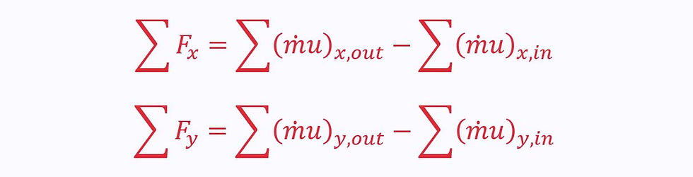
Even though one of the velocity vectors dots with the area vector to become a scalar, the second velocity vector remains. Therefore, the equation needs to be split into components, u and v:


This can be interpreted to mean the sum of forces in a particular direction is equal to the momentum outflow minus the momentum inflow in that direction.
As seen in the notes sheet of forces in fluids, all fluids consist of body and surface forces.
All body forces in the control volume (e.g., weight) must be accounted for.
Only the surface forces at the control volume boundary, however, must be taken account for here (as internal forces cancel out).
These could be atmospheric pressure or reaction forces.
Algebraic Formulation
The integrated form of the conservation of momentum equation above is not all that useful. Instead, if velocity is uniform at an inlet or outlet, this inlet or outlet can be looked at individually.
The surface integral for the whole control volume therefore becomes an area integral for just that inlet/outlet:

(See mass flow rate above)
Therefore, the conservation of momentum can be written in terms of the sum of all outlet momentums minus those at the inlets:
For one inlet and one outlet:

Using conservation of mass:


Comments